
Background
For this project, I will be using the California Safe Cosmetics Program (CSCP) dataset from the California Department of Public Health. This is a dataset intended for public access and use which can be found here.
The CSCP’s aim is to compile a list of cosmetic products that contain hazardous ingredients known/suspected of causing cancer, birth defects, or developmental and reproductive harm. The California Safe Cosmetics Act (2005) and Cosmetic Fragrance Ingredient Right to Know Act (2020) require that all harmful ingredients listed on labels must be reported to the California Department of Public Health to be compiled into a list for public disclosure.
This article is part II of a two part series. Part I discussed the creation of business rules and an entity relationship diagram for the CSCP dataset. Part II focuses on building the relational database.
If you are interested in following along with my process, check out my CSCP GitHub repository for metadata, raw data, cleaned tables and more.
Introduction to Data Cleaning & Data Wrangling
What is the first image that comes to mind when you read the phrases “data cleaning” and “data wrangling”?
I think of a sink of dirty dishes. There’s flecks of old food on the plates and coffee residue in mugs. You decide to tackle the top dishes first so that you can avoid sticking your hands in some unknown mess at the bottom of the pile. After you scrub and rinse off each dish, they are placed in the dishwasher in orderly rows.
Can you guess which process is which?
Data cleaning is similar to when you scrub food off a dirty plate. Leaving leftover food on the dishes could clog your dish washer, leading to a high repair cost. Poorly cleaned data can lead to bad decision making, costing companies time, resources, and money to correct. Removing and-or modifying errors and irrelevant entires in messy data can prevent these disastrous outcomes.
Data wrangling the sink of dirty dishes would involve organizing dishes to fit neatly in the dishwasher. Throwing all dishes in randomly is inefficient time and space-wise. The same goes for data. By wrangling the data, we can transform it from raw data into a useable format for downstream analysis.
If you guessed the processes correctly, great job!
Now onto the tricky part: what process do you tackle first?
Searching the internet for the order of operations for data cleaning and data wrangling results in a chicken-and-the-egg conundrum. Some sources state that cleaning comes first before restructuring the data [1]. Others view cleaning data as a nested process of data wrangling[2].
I like to think of data cleaning and data wrangling as more of a fluid process. It’s that dreaded answer of… “Well it depends.” The processes are complementary, their order depends on the goals of the project and the data itself [1].
Cleaning and Wrangling the CSCP dataset
For Part II of California Safe Cosmetics Program (CSCP) project, my goal was to develop a relational database ready for analysis. By definition, a relational database is composed of structured tables that are connected to one another by relationships.
Remember the entity relationship diagram (ERD) we built in Part I?
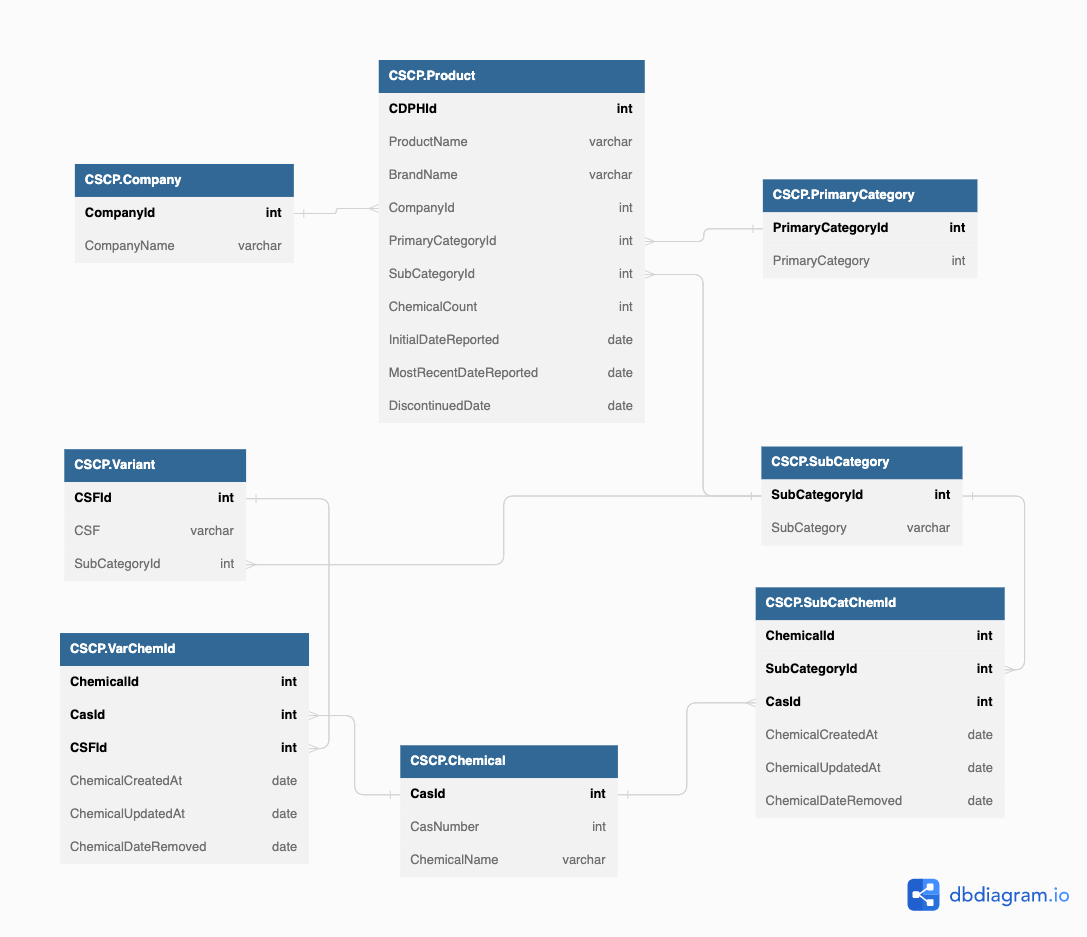
Using this ERD as a guide, we can start the data cleaning and wrangling process. The bolded attributes in each rectangle are primary keys. As primary keys, each row must have a distinct identifier.
However, since the CSCP dataset is a spreadsheet, its difficult to immediately parse the distinct identifiers of the future tables. That’s why data cleaning and data wrangling are used simultaneously for this project.
The first step is to wrangle the tables to match the attributes listed in each of the entity boxes. The Chemical, SubCategory, PrimaryCategory, Product, and Company tables contain a singular unique primary key. Thus, for these tables we can remove duplicate entries in R before exporting them into Excel for data cleaning.
As for the Variant, SubCatChemID, and VarChemID tables, we have to do a little more wrangling legwork.
Let’s start with the Variant and VarChemID tables. The Variant table has CSFIds as the primary key. Since primary keys cannot have null values, we have to remove all CSFIds that are nulls before creating the Variant table.
ch_df_v2 <- ch_df
ch_df_v2$CSFId[which(is.na(ch_df_v2$CSFId) == T)]<-0
ch_df_v2 <- ch_df_v2[!(ch_df_v2$CSFId == 0),]
Pretty easy right?
The VarChemID table has the CSFId as a foreign key, so we can also use the ch_df_v2 dataset to build this table.
The SubCatChemId table is a bit tougher. It’s the alternate reality of the Variant table where all product chemicals have CSFIds that are nulls. We have to put a value of ’T’ into the CSFID nulls so that we can subset and create this table.
ch_df_v3 <- ch_df
ch_df_v3$CSFId[which(is.na(ch_df_v3$CSFId) == T)]<-'T'
ch_df_v4 <- ch_df_v3[which(ch_df_v3$CSFId=='T'),]
Ok, now we have some messy relational tables. We can import the tables into Excel to begin the cleaning process.
Data Cleaning Framework
For the section, I will discuss the data cleaning process using a six step framework [3].
Remove Irrelevant Data to your Business Problem
Since we are building a database, data is relevant to its assigned table. An example of irrelevance would be if the CompanyName was assigned to the Chemical table. This step is completed in conjunction with data wrangling.
Remove Duplicate Primary Keys
For parent tables with a singular primary key, duplicates can be removed early in the data wrangling process. However, if child tables contain foreign keys, duplicates must be removed after the parent tables’ primary keys have been standardized.
Search and Repair Structural Errors
Repairing structural errors such as misspellings and poor naming conventions took the most time to complete. This is why I wrangled the relational tables prior to cleaning. Sorting the names in ascending order, the smaller datasets made it easier to see structural errors.
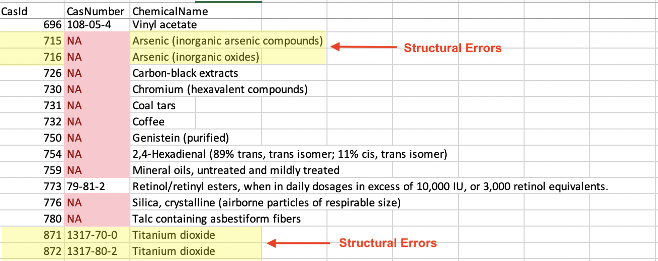
I standardized the naming conventions manually by consolidating entries into a singular name. For example, in the unsorted Chemical table, we can see that Arsenic has two different names: ‘Arsenic (inorganic arsenic compounds)’ and ‘Arsenic (inorganic oxides)’. They were given different CasIds as if they were different chemicals. The ChemicalName and CasID need to be corrected for accurate downstream analysis.
Listing the primary key CasIds of the consolidated name (ex. Arsenic has CasIDs of 715 and 716), we can designate one identification number and delete the other iterations of the CasId. We can standardize these ids using two methods: through ’Find and Replace’ in Excel or building a function in R.
After trying both methods, I found R to be the superior option. R was more efficient than Excel at changing values. It also mitigated the human-error risk of clicking “Replace all” which can alter data outside of the specified column. Here’s the R-function for curious folks:
df1$column2[df1$column2 == old-number2] <- new-number
df1[grep(old-number2, df1$column2),]
Grep checks to see if all ‘old numbers’ were successfully replaced. This is part of validation, which I discuss later!
Another structural error seen in the Chemical table was that ChemicalName was not specific enough to CasNumber. Googling the CasNumber, we can find and input the correct ChemicalName into the spreadsheet.
This process was repeated for each table. After the primary key errors were repaired for the Company, Primary Category, SubCategory, and Chemical parent tables, the child tables’ (Product and Variant) and the bridge tables’ (VarChemID and SubCatChemID) foreign keys can be repaired.
With all of the primary keys and foreign keys tidied up, we can remove duplicates from the VarChemID and SubCatChemID composite keys using the ‘Remove duplicates’ function in Excel.
Fix Missing Data
There are a few ways to fix missing data. You can:
Search the internet if the missing value is a static definition.
Restructure the data to prevent issues by choosing a different primary key.
Eliminate the data entirely.
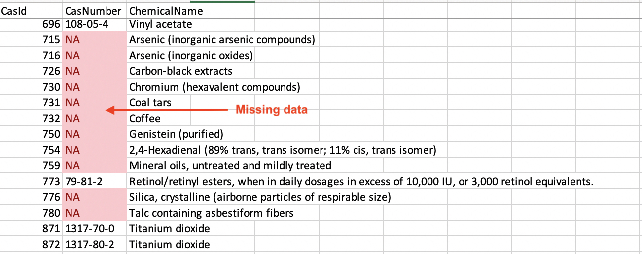
I highlighted fields with NAs using conditional formatting in Excel. Luckily the missing data in the CSCP dataset was easily searchable online. This improved the robustness of the dataset.
Outliers
Data that falls outside of the norm are called outliers. This data can skew analyses resulting in inaccurate insights and poor decision making.
Since this project’s focus was to build the CSCP relational database, we don’t have to worry about this step right now.
Data Validation
The last step is to check if the data is ready for downstream analyses. We already validated the structural changes using grep in R earlier. During validation, we examine the the data for consistency and proper formatting.
As the final check, I uploaded the tables into Tableau to confirm the primary-foreign key relationships.
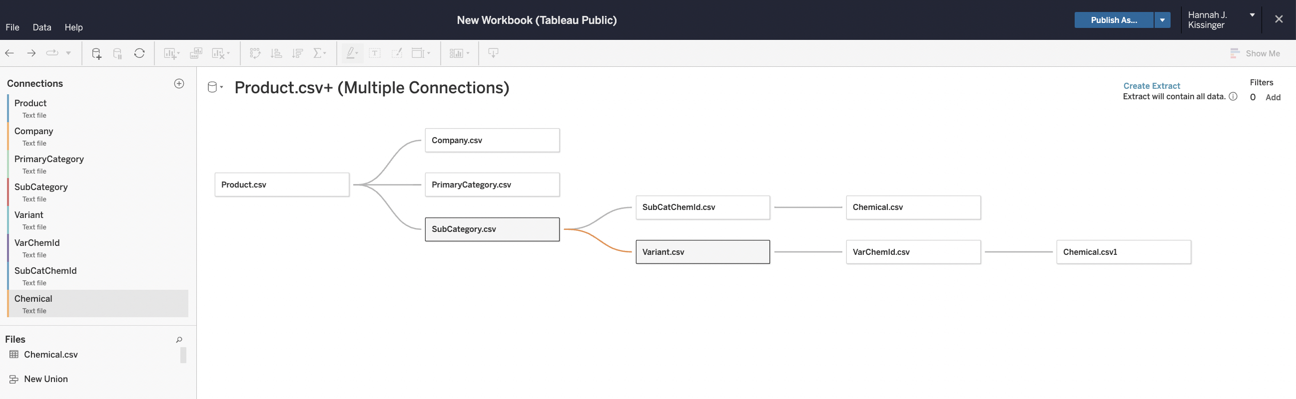
It worked! Now that we have a relational database we can move onto analysis!
Conclusion
As you can see, data wrangling and data cleaning can be very fluid processes when building a relational database. To see all of the changes made check out the changelog and R-Scripts in my GitHub repository.
Now that we understand the relationships between entities (Part I) and built the relational database in Part II.
Citations
[1] Todd, S. (2020). Data Wrangling Vs. Data Cleaning, What’s the Difference?. URL: https://www.inzata.com/data-wrangling-vs-data-cleaning-whats-the-difference/#:~:text=Traditionally%2C%20data%20cleaning%20would%20be,maximize%20the%20value%20of%20insights.
[2] Kirsch, K. (2021). What’s the Difference Between Data Wrangling vs Data Cleansing vs Data Transformations. URL: https://www.osmos.io/blog/data-wrangling-vs-data-cleansing-vs-data-transformations
[3] Mesevage, T.G. (2021). Cleaning Steps & Process to Prep Your Data for Success. URL: https://monkeylearn.com/blog/data-cleaning-steps/